I have fully transferred my blogs to http://app186.blogspot.com/. Sorry for the trouble..
I am sorry ma'am but I need to transfer my blog to blogspot because I cannot upload my images using the connection in NIP. I don't know why. Click here for the link of my new blog for Activities 3 onwards. I will be transferring the previous two activities into that blog the soonest possible time. Thank you!
Another activity has passed and here I am again saying to you about this. I have a few difficulty encountered as I do this activity but I conquered this difficulty and applied the basics of Scilab to gain points for this activity. The activity has 6 items to do. Below are the activities that were done for Activity 2.

Figure 1. Centered circular aperture or pinhole
Here, I have placed a circular aperture on the center of the image. This part is a practice in order to familiarize the codes in using scilab. The code below is the code
of this figure:
of this figure:
- nx = 100; ny = 100; //defines the number of elements along x and y
- x = linspace(-1, 1, nx); //defines the range
- y = linspace (-1, 1, ny);
- [X, Y] = ndgrid(x,y); //creates two 2D arrays of x and y coordinates
- r = sqrt(X.^2 + Y.^2);//note: element per element squaring of X and Y
- A = zeros(nx,ny); //creating a nx-by-ny matrix
- A(find(r<0.7)) = 1;
- imshow(A);
- imwrite(A, "C:\Users\MP\Documents\Dropbox\Files\186\A2 - Circles.jpg");

Figure 2. Centered square aperture or pinhole
The figure above is somewhat difficult for me. At first I did not understand how it can be created but after several trials, I have created figure 3. At first it was only one horizontal white rectangle in the middle. It made me think that maybe scilab has the &-property wherein both statement are true before the command will proceed. And with that, I have created a square aperture located in the center. Below is the code for the square aperture:
- nx = 100; ny = 100; //defines the number of elements along x and y
- x = linspace(-1, 1, nx); //defines the range
- y = linspace (-1, 1, ny);
- [X, Y] = ndgrid(x,y); //creates two 2D arrays of x and y coordinates
- A = zeros(nx, ny);
- A(find(abs(X) < 0.4 & abs(Y) < 0.4)) = 1;
- imshow(A);
- imwrite(A, "C:\Users\MP\Documents\Dropbox\Files\186\A2 - Square.jpg");

Figure 3. Sinusoid along the x-axis(Corrugated roof)
I do not know whether the figure above is correct or not. I simply place a sine wave into the X - axis values and there it is. It just popped up like it is correct. I guess it is correct. Below is the code I have created for this figure.
- nx = 100; ny = 100; //defines the number of elements along x and y
- x = linspace(-1, 1, nx); //defines the range
- y = linspace (-1, 1, ny);
- [X, Y] = ndgrid(x,y); //creates two 2D arrays of x and y coordinates
- cr = sin(X * 6 * %pi) //%pi is 3.1415
- imshow(cr);
- imwrite(cr, "C:\Users\MP\Documents\Dropbox\Files\186\A2 - Sinusoid.jpg");

Figure 4. Grating
This one is the easiest part that I have done. There is no instruction in how far should the spacing of this grating should be so I assumed to be one space after another. Below is the code I have written in making a grating.
- nx = 100; ny = 100; //defines the number of elements along x and y
- x = linspace(-1, 1, nx); //defines the range
- y = linspace (-1, 1, ny);
- [X, Y] = ndgrid(x,y); //creates two 2D arrays of x and y coordinates
- A = zeros(nx, ny);
- for i = 1:2:nx
- A(i,:) = 1;
- end
- imshow(A);
- imwrite(A, "C:\Users\MP\Documents\Dropbox\Files\186\A2 - Grating.jpg");
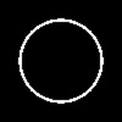
Figure 5. Annulus
This one is as simple as the practice part. Aside from looking for the indices of small value, I made a range of values of the circle so that an annulus is formed. This is like an absolute value, i.e. |x| < 1 ===> -1 < x < 1. Below is the code for the annulus.
- nx = 100; ny = 100; //defines the number of elements along x and y
- x = linspace(-1, 1, nx); //defines the range
- y = linspace (-1, 1, ny);
- [X, Y] = ndgrid(x,y); //creates two 2D arrays of x and y coordinates
- r = sqrt(X.^2 + Y.^2);//note: element per element squaring of X and Y
- A = zeros(nx,ny); //creating a nx-by-ny matrix
- A( find( r < 0.7 & r > 0.65 ) ) = 1;
- imshow(A);
- imwrite(A, "C:\Users\MP\Documents\Dropbox\Files\186\A2 - Annulus.jpg");
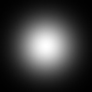
Figure 6. Circular aperture with graded transparency
I happened to know how to do this one since I am making one of this for my research. It is simply having a grid values X and Y then placing it into the equation for the Gaussian Distribution. Below is the code I have made.
- nx = 100; ny = 100; //defines the number of elements along x and y
- x = linspace(-1, 1, nx); //defines the range
- y = linspace (-1, 1, ny);
- [X, Y] = ndgrid(x,y); //creates two 2D arrays of x and y coordinates
- sigma = 0.4;
- r = 1/sqrt( 2 * %pi * sigma^2) * exp( -0.5 * ( X.^2 + Y.^2) / sigma^2); //Gaussian distribution
- imshow(r);
- imwrite(r, "C:\Users\MP\Documents\Dropbox\Files\186\A2 - Aperture.jpg");
I have done this activity last Friday, 17 June 2011. I am not that in a hurry. It's just that I have a vacant time that I have nothing else to do. I will rate myself with 5 for technical corrections since I can see that I have done no error for this activity. Another 5 for Presentation quality because I have placed the figures with their captions and also the codes I have made in creating those figures. And for the Initiative part, I have given myself 2 points because I have used the formula of the Gaussian distribution and the logic & in getting the square in the middle.
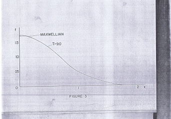
Figure 1. Scanned hand-drawn plot in a 1970s thesis located in NIP Library.
Here I am, writing a blog for my class. I don't why I have to do this but I have to do this blog right now. I am done in duplicating the graph I have. The image above is the one I have gotten from a thesis from 1970. The picture below is the graph I have attempted in duplicating the picture above.
As you can see, the plot I have created with the red-colored line almost coincide with the graph that I have chosen. I have not duplicated the entire plot due to it's rotation that I have done with the help of James Christopher Pang and GIMP. :)
It was difficult to do the approximations using only the PAINT program. It has features that was not there in order to rotate the image because the plot is not straight and so the pixel of a straight vertical line varies. After rotating the graph, it looks like a good graph already and so I superimpose the rotated image and the plot that I have and poof, the lines almost coincide.
I am happy with what I have done. I am sure I have done a good job in doing the activity. So I guess, I will rate myself with 4 for the Technical Corrections because the figure I have has still some corrections and it's not exactly the same, 4 for Quality of Presentation because it has few errors in the figure, 2 for the Initiatives because I have used another software in order to have a more accurate figure to duplicate.
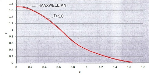
Figure 2. Duplicated plot with the red line as the duplicate line and the sample is the dark line.