Another activity has passed and here I am again saying to you about this. I have a few difficulty encountered as I do this activity but I conquered this difficulty and applied the basics of Scilab to gain points for this activity. The activity has 6 items to do. Below are the activities that were done for Activity 2.

Figure 1. Centered circular aperture or pinhole
Here, I have placed a circular aperture on the center of the image. This part is a practice in order to familiarize the codes in using scilab. The code below is the code
of this figure:
of this figure:
- nx = 100; ny = 100; //defines the number of elements along x and y
- x = linspace(-1, 1, nx); //defines the range
- y = linspace (-1, 1, ny);
- [X, Y] = ndgrid(x,y); //creates two 2D arrays of x and y coordinates
- r = sqrt(X.^2 + Y.^2);//note: element per element squaring of X and Y
- A = zeros(nx,ny); //creating a nx-by-ny matrix
- A(find(r<0.7)) = 1;
- imshow(A);
- imwrite(A, "C:\Users\MP\Documents\Dropbox\Files\186\A2 - Circles.jpg");

Figure 2. Centered square aperture or pinhole
The figure above is somewhat difficult for me. At first I did not understand how it can be created but after several trials, I have created figure 3. At first it was only one horizontal white rectangle in the middle. It made me think that maybe scilab has the &-property wherein both statement are true before the command will proceed. And with that, I have created a square aperture located in the center. Below is the code for the square aperture:
- nx = 100; ny = 100; //defines the number of elements along x and y
- x = linspace(-1, 1, nx); //defines the range
- y = linspace (-1, 1, ny);
- [X, Y] = ndgrid(x,y); //creates two 2D arrays of x and y coordinates
- A = zeros(nx, ny);
- A(find(abs(X) < 0.4 & abs(Y) < 0.4)) = 1;
- imshow(A);
- imwrite(A, "C:\Users\MP\Documents\Dropbox\Files\186\A2 - Square.jpg");

Figure 3. Sinusoid along the x-axis(Corrugated roof)
I do not know whether the figure above is correct or not. I simply place a sine wave into the X - axis values and there it is. It just popped up like it is correct. I guess it is correct. Below is the code I have created for this figure.
- nx = 100; ny = 100; //defines the number of elements along x and y
- x = linspace(-1, 1, nx); //defines the range
- y = linspace (-1, 1, ny);
- [X, Y] = ndgrid(x,y); //creates two 2D arrays of x and y coordinates
- cr = sin(X * 6 * %pi) //%pi is 3.1415
- imshow(cr);
- imwrite(cr, "C:\Users\MP\Documents\Dropbox\Files\186\A2 - Sinusoid.jpg");
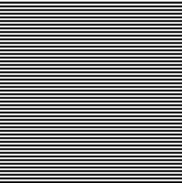
Figure 4. Grating
This one is the easiest part that I have done. There is no instruction in how far should the spacing of this grating should be so I assumed to be one space after another. Below is the code I have written in making a grating.
- nx = 100; ny = 100; //defines the number of elements along x and y
- x = linspace(-1, 1, nx); //defines the range
- y = linspace (-1, 1, ny);
- [X, Y] = ndgrid(x,y); //creates two 2D arrays of x and y coordinates
- A = zeros(nx, ny);
- for i = 1:2:nx
- A(i,:) = 1;
- end
- imshow(A);
- imwrite(A, "C:\Users\MP\Documents\Dropbox\Files\186\A2 - Grating.jpg");
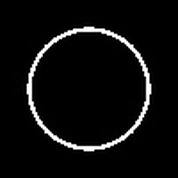
Figure 5. Annulus
This one is as simple as the practice part. Aside from looking for the indices of small value, I made a range of values of the circle so that an annulus is formed. This is like an absolute value, i.e. |x| < 1 ===> -1 < x < 1. Below is the code for the annulus.
- nx = 100; ny = 100; //defines the number of elements along x and y
- x = linspace(-1, 1, nx); //defines the range
- y = linspace (-1, 1, ny);
- [X, Y] = ndgrid(x,y); //creates two 2D arrays of x and y coordinates
- r = sqrt(X.^2 + Y.^2);//note: element per element squaring of X and Y
- A = zeros(nx,ny); //creating a nx-by-ny matrix
- A( find( r < 0.7 & r > 0.65 ) ) = 1;
- imshow(A);
- imwrite(A, "C:\Users\MP\Documents\Dropbox\Files\186\A2 - Annulus.jpg");
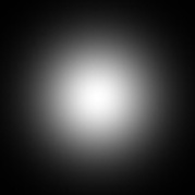
Figure 6. Circular aperture with graded transparency
I happened to know how to do this one since I am making one of this for my research. It is simply having a grid values X and Y then placing it into the equation for the Gaussian Distribution. Below is the code I have made.
- nx = 100; ny = 100; //defines the number of elements along x and y
- x = linspace(-1, 1, nx); //defines the range
- y = linspace (-1, 1, ny);
- [X, Y] = ndgrid(x,y); //creates two 2D arrays of x and y coordinates
- sigma = 0.4;
- r = 1/sqrt( 2 * %pi * sigma^2) * exp( -0.5 * ( X.^2 + Y.^2) / sigma^2); //Gaussian distribution
- imshow(r);
- imwrite(r, "C:\Users\MP\Documents\Dropbox\Files\186\A2 - Aperture.jpg");
I have done this activity last Friday, 17 June 2011. I am not that in a hurry. It's just that I have a vacant time that I have nothing else to do. I will rate myself with 5 for technical corrections since I can see that I have done no error for this activity. Another 5 for Presentation quality because I have placed the figures with their captions and also the codes I have made in creating those figures. And for the Initiative part, I have given myself 2 points because I have used the formula of the Gaussian distribution and the logic & in getting the square in the middle.